This is an old revision of the document!
From zero to tomato
In this class we start with installing GroIMP and move forward towards our very first light sensitive tomato plant.
This class consists of the following tutorials:
Install with executable file
The easiest way to install GroIMP is to run an executable file. The executable file is downloadable on the grogra website. It can then be executed like many common installer file by double clicking on it. This trigger the installation of the software. The file will also automatically create a shortcut.
Requirements
GroIMP is written in Java, which means it should follow Java's WORA-principle (Write Once, Run Anywhere) and should run on every Java-capable platform. GroIMP has been tested successfully on Mac, Linux and Windows platforms.
GroIMP 2.2 requires the installation of a Java runtime environment of version 21. This can be obtained from Oracle at https://www.oracle.com/de/java/technologies/downloads/#java21.
For a reasonably performant runtime behaviour, at least 256 MB RAM and a 1 GHz processor are recommended.
Download
GroIMP installation executable are available on the grogra website and on the gitlab release section as a zip-file, windows exe, or debian release.
Run the installation
Windows
The windows exe is an executable file that will extract and install GroIMP on your computer.
While you are downloading the file you might get some warning from your web browser that the software is not certified by Microsoft. Please ignore this warning, as we neither had the funding nor the time to go through the certification process.
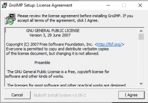
Please double click on the downloaded file (make sure you have administrator rights on your machine for installation), and follow the instructions one by one:
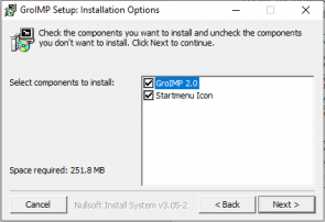
Normally, click on ‘I Agree’, then on ‘Next’. Choose the destination folder, then the maximum heap size for Java. This allocates a certain amount of RAM (random access memory) to the Java Virtual Machine on which GroIMP is running. By default, 1500 MB are allocated, but you can allocate up to 50 per cent of the RAM available on your machine to Java, without any problem (so on a machine with 10 GB RAM you can enter 5000):


After this you click on ‘Install’ and wait for the installation to finish (this can take more than ten minutes).
After the installation, a folder “GroIMP-2.2” should be available under something like this address: “C:\Program Files\”.
GroIMP will now be available either on your desktop or in the list of programmes:
Mac OS
Mac users need to download the zip-file, extract it and run GroIMP from the command line.
The directory structure of the zip-file has to be preserved, check that your zip program is set up accordingly (and does not extract all files into one and the same directory).
After extraction of the zip-file, the following files, amongst others, are present in the installation directory:
`README`
This plain text file contains additional information about the GroIMP distribution. Please read it carefully.
`INSTALL`
This plain text file contains instructions for the installation of the GroIMP distribution, legal notices and other information. Please read it carefully. If you have trouble with the installation procedure described in this manual, please consult the file `INSTALL` for a solution.
`plugins`
This directory contains all the plugins that are part of the binary distribution of GroIMP.
`core.jar`
This file is an executable java archive and the entry-point for the Java runtime environment to start the GroIMP application.
Ubuntu & Debian
The .deb file is an executable file that will extract and install GroIMP on your computer.
In most modern Ubuntu systems you can just click on the downloaded deb file and it will open the package manager which allows you to install the software.
If this is not possible you can use sudo dpkg -i /path/to/groimp.deb in a command line.
Increasing heap space on Linux
If you want to start GroIMP with additional heap space you can do so from the command line:
groimp -Xmx Xmx5G
Others
As a java software it is possible to execute GroIMP on any system that can run a java virtual machine of version 21. This includes almost any version of Linux as well as some other systems. For this case we provide an archive with the compiled jar on the Gitlab release page. This can then be executed with java -jar core.jar
Running GroIMP
Because `core.jar` is an executable java archive, it is possible to start GroIMP just by (double-)clicking on the file in your system's file browser as you would do with a usual executable file. This requires a suitable setup of your file browser, see the documentation of the browser and your Java installation if it does not already work.
From a Shortcut
You can set up your desktop to show a menu entry for GroIMP. How this is done depends on your system. Usually your system provides a menu editor where you can create a new menu entry and specifiy the command to be executed when the entry is activated. Choose the command as you would do on command line.
From the Command Line
The file `core.jar` in your installation directory of GroIMP's binary distribution is the entry-point for starting GroIMP. Running GroIMP from the command line is easy:
java -jar path/to/core.jar
Of course, `path/to/core.jar` has to be replaced by the actual path to the file `core.jar`. E.g., if, on a Unix system, the installation directory is `/usr/lib/groimp`, the command would be
java -jar /usr/lib/groimp/core.jar
or, on a Windows system with installation directory `C:\Program Files\GroIMP`,
java -Xverify:none -jar “C:\\Program Files\\GroIMP\\core.jar”
Alternatively, if you wish to start GroIMP from a batch file from your cmd console in Windows, you could write a file called groimp.bat (which you would place in your home directory, C:\\Users\\myself\\, where 'myself' is your user directory) with the following content:
cd “C:\Program Files\GroIMP 2.1.5”
“C:\Program Files\Java\jdk-22\bin\javaw.exe” -Xmx3000m -Xss20M -noverify -jar core.jar
where “C:\Program Files\Java\jdk-22\bin\javaw.exe” is an example of the placement of your javaw version, assuming we use jdk22.
GroIMP Interfaces
See GroIMP interfaces for more details.
GroIMP can be run from different interfaces. By default, GroIMP use the “imp” interface which is its Graphical User Interface (GUI).
GroIMP can also be started headless, from CLI, or API.
To define which interface is used, when starting GroIMP you need to pass the parameter -a. E.g.
> java -jar core.jar -a api
More information can be found for using GroIMP headless, CLI, and API.
Run first model
After you followed the installation instruction and started the software, you should be able to proceed the steps shown in the animation below:

Running your first RGG model
Installation
GroIMP is a Java-based application that supports Windows, Mac and Linux. Installation files can be found here.
Before installing GroIMP, please make sure that you have Java 21 or higher installed on your computer. If not you can find the oracle version here. It is possible to have several Java versions on your device, please make sure that GroIMP uses the right one.
Additional information can be found in the tutorials: Installing GroIMP After installing GroIMP using an installer, a desktop shortcut is provided that starts the GUI, for more information and troubleshooting see Running GroIMP
Look around
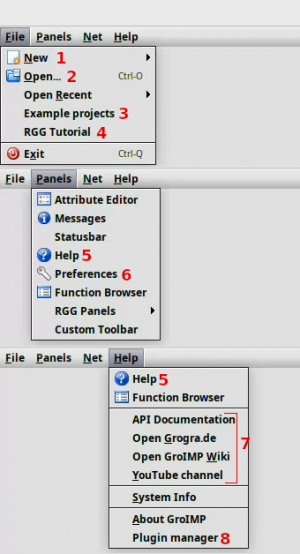
On the first window, even though it is empty, we can already find some important parts of the software, especially for finding help and getting started.
- New creates a new GroIMP project from one of the templates - we are going to use this in the next step
- Open allows you to open GroIMP projects. These are stored either as gsz or gs files.
- Example projects provides you with a collection of embedded example projects that try to highlight the most important features of the software. More examples can be found online in our gallery.
- The RGG Tutorial is an embedded tutorial that gives an interactive introduction to the XL/RGG syntax
- Help opens the embedded documentation of all the installed plugins.
- Under Preferences most GroIMP features can be customized, from rendering, over the number of buttons on a toolbar, to the ports of the embedded servers. This is documented here.
- This part of the menu points to several helpful webpages that provide various information:
- The API Documentation provides the javadoc of GroIMP: Though very confusing at first glance, it is nevertheless potentially very helpful once you dive deeper into modelling with GroIMP because it allows you to know what each class can do and how classes are related to each other.
- Grogra.de is the main page of our project
- GroIMP wiki The GroIMP wiki (you are on it right now) is a collection of tutorials and descriptions of the different parts of the software.
- The GroIMP youtube channel can give you some inspiration of what to do with GroIMP (and what others already produced with it)
- With the Plugin Manager it is possible to install, remove and update plugins (parts of the software). This is documented here
New RGG
First of all, to get a first impression of modelling in GroIMP, let's open our first RGG project. To do so, go to the menu, click on New (the 1 in the image above) and select “RGG Project”.
This will provide you with the following window:

Let's have a short look around:
- The RGG toolbar provides a button for each public function in the RGG code (the code can be seen in the code editor(4)); if you wish you can click on run and see the changes in the 3D view. Additionally, it comes with a reset button, which brings the simulation back to the starting point (defined in the init function).
- The 3D view shows the current state of the model. It is possible to navigate through the model using either mouse control or the navigation button on the top right. With the menu it is possible to customize the view and the camera and to render the view with different renderers. Additionally, in the menu under View /export you can export the 3d scene in several formats. The 3D view is also used to select and edit objects in the scene as shown on the right. When selected the attribute editor (7) is opened.
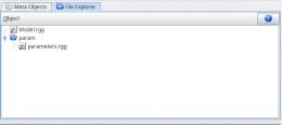
- A GroIMP model is coded in the RGG programming language, and the code is stored in files with the extension rgg. To manage the files the File Explorer is used, here you can add, create and delete files and folders. To create a file you have to add a not yet existing file. If you select a file it is opened in the code editor (4) you can try this with the parameters.rgg file in the folder param.
- GroIMP includes the code editor jEdit to edit the source files of the simulation. If not changed in the preferences, pressing Ctrl-s will save the code and recompile and reset your simulation. Try this by changing setShader(GREEN) to setShader(BLUE) in the file Model.rgg and save. This should turn our little sphere blue.
- If, for example, you mis-type setShader(BLUH) (instead of BLUE) you will see an error message in the messages panel. This panel will give you information about most events and issues in your project.
- Each file you create in your model is compiled and added to the Meta Objects explorer. If you select one here it opens the attribute editor (7) for the model.
- The Attribute editor can be used to manipulate the currently selected objects. This includes the nodes and the meta objects. If, for instance, you select the little sphere, change the field Radius and press enter the selected sphere is changing the diameter. However, if you click reset on the RGG toolbar(1) the sphere (actually a new version of it) returns to its original size (since the init() method has now been executed).
- Finally, the XL-Console is used to run RGG commands on the model without recompiling it, which can be helpful for analyzing or manipulating the model during a simulation. Try to type
((*Model.A*)), that will list you all A's in your simulation. If you press the run button in the RGG toolbar(1) and run the command in the console again there will be more output. On the right you can see a history of the last commands you used. Why can't we simply write((*A*))? Try it, and you will see an error message. In fact, the XL console is outside of the Model (which is an RGG class), so we need to tell GroIMP that we want to access the module A that only exists in Model.rgg.
Additional panels
Beside the panels opened directly in the beginning there are several others that can help you at times. Here are two panels that may get you started:
- /Panels/2D/Graph : provides you with a visual representation of your simulation graph. This is very helpful to understand the theoretical background of GroIMP. Also it allows you to select nodes that are not visible.
- /Help/Function Browser : can help you to identify or find functions used in RGG, this can help you especially in the beginning to understand models of other users.
Saving
To save your project, you can either press the save button in the RGG toolbar or go to File/Save. This provides you with a file dialog where you can select a location to save. The possible file types are .gs and .gsz. The simplest to use is gsz, which creates just one archive of all the files and saves it. This can then be moved and shared. The gs option saves the same files, but they will not be compressed, which means the project is a whole folder.
RGG Code structure introduction
The RGG programming language repents the core of almost all GroIMP models. This language extends java and implements the XL-language specification (https://manual.grogra.de/XL/index.html), to enable rule based graph manipulation.
This leads to a programming language based on two paradigms, the object orientation of java and the rule based structure of XL. In order to separate these two rgg is using different brackets to define code blocks.
The java blocks are framed by curly brackets {…} and the xl blocks by square brackets […]. These blocks can be embedded into each other recursively and share declared variables.
Functions
Even so the function declaration follows the syntax of java, the body of the function can be of both code blocks. In difference to java rgg code allows to start directly with the declaration of functions without creating a class before. (Internally the rgg file is handled as one java class).
If a function is defined by public void and needs no parameters, it is automatically added to the RGG toolbar after compilation (the list of buttons above the 3d view). This functions are the main way to interact with a running RGG simulation.
init
Additionally there are several functions predefined that can be used to change the behavior of the simulation. At this point we will only talk about the initialization: protected void init (). this function is executed after the compilation or a model reset.
protected void init ()
[
	{println("hallo");}
	Axiom ==> A(parameters.length);
]
The Axiom is the node that is added to the graph in the very beginning of the simulation and is used as an access point.
Java blocks
The java block allow java syntax up to java 1.6. (this is independent from the java version that is used to run GroIMP). Therefore it is possible to use features such as file reading and writing, mathematical calculations, abstraction/inheritance or library functions. If you are not experienced with java it might be useful for you to look into available online tutorials.(For example https://www.w3schools.com/java/default.asp)
Every new rgg file also imports by default a set of library functions that are used to interact with the graph or the GroIMP platform. This functions can be explored in the function explorer in the software. You can find it on the main menu under 'Help/Function Browser'.
Moreover rgg comes with some additions to the java syntax, or more accurate to the syntax of java 6.
Modules
A module in RGG is very similar to a class in java, it can extend other modules or implements java interfaces. It can also hold functions like 'getDiameter()' in the example below. One large difference is that a in a module the constructor is different. The parameters are unlink in a java class directly defined in the head of the module (see below 'float len') and the code executed on the initialization of a module is defined by just a second par of curly brackets (see below {setShader(GREEN);}).
Besides that the main difference is the use case. A module is always a GroIMP Node, meaning it can be added to the GroIMP simulation graph (ProjectGraph) similar to turtle commands or the base 3d Objects.
module A(float len) extends Sphere(0.1)
{
	{setShader(GREEN);}

	public float getDiameter(){
		return radius*2;
	}
}
Its syntax is simple and provisional, changes or extensions are likely to occur.
The simplest form of a module declaration is
module SimpleModule;
which declares a module of name SimpleModule with no fields. These simple modules can be useful for aggregations, multi scaling or just as place holders.
The addition of fields is done as in
module ModuleWithFields (int type, String name);
If o is an instance of ModuleWithFields, the usual Java syntax o.type can be used to access a field. This form of a module declaration provides a constructor with parameters corresponding to the specified module parameters.
A module is a part of the Java class hierarchy. It is possible for a module to be a subclass of another class or module, this is indicated by an extends-clause:
module Sub (super.type, super.name, int extra) extends ModuleWithFields;
The module Sub is a subclass (submodule) of ModuleWithFields. The fields type and name are inherited from ModuleWithFields, extra is a new field. A constructor having three parameters (type, name, extra) is provided. It looks for a superclass constructor applicable to the inherited arguments type, name of type int, String (which is found in ModuleWithFields).
Sometimes, not all module parameters are to be inherited. In these cases, one has to specify the superclass constructor to be used by explicitly providing its arguments as in
module Sub2 (super.name) extends ModuleWithFields (1, name);
Instantiation
While in theory every part/organ/etc… of the simulated object (normally a plant) is suppose to be represented in the graph, it is not allays suitable to add all geometrical objects that represent an object individually. Therefore the concept of instantiations was included. Using the syntax below the module Branch is one object in the graph and is during the creation of the object interpreted as an extension of M. Yet for the visualization and the ray tracing it is represented by the four F objects with the different shaders.
module Branch(float len) extends M(len)==>
     F(len/4).(setShader(GREEN))
     F(len/4).(setShader(BLUE))
     F(len/4).(setShader(GREEN))
     F(len/4).(setShader(BLUE));
On the right side of the ==> operator a syntax similar to the production part of a rule can be used.
It has to be noticed that even so instantiations create a smaller graph they tempt to slow down the visualization.
Queries
In GroIMP the project graph is considered to hold almost all information on the simulation. Therefore it can also be seen as a knowledge graph. To retrieve this knowledge rgg uses the XL query system. To use this queries in a java block they have to be framed by (*…*) as shown in the examples below. In that way they return a collection object, which then can be like other java objects. Moreover GroIMP comes with a set of predefined Analytical methods to analyze this collections.
As shown in the example below in count((*M*)) this queries work with the concept of java objects. Therefore (*M*) is selecting all instances of Branch because Branch extends M. This also works with interfaces.
public void calc(){
	long countA = count((*RU(30) RH(90) A*));
	long countM = count((*M*));
	if(countM>0){
		println((float)countA/(float)countM);
	}
	println(sum((*Branch*).len));
}
in the last line of the example above: println(sum((*Branch*).len)); one way to access attributes (or functions) of modules is shown. The other way is shown below in: (*A*)[radius]+=0.1; .
The first way is more in the style of java while the second way is better adapted to GroIMP. Therefore the second way is not only changing the attribute of the object but also notifies the change to the platform.
Moreover it manages the access of the attributes differently, (for instance would (*A*).radius not be allowed because radius is not accessible in a java way.
public void growRadius(){
	(*A*)[radius]+=0.1;
}
Lambda expressions
Since java 1.6 did not include lamda expression, an own implementation was added to rgg. The syntax an the explanation can be found here
XL Blocks - Rules
While using XL queries mainly three rules are used:
- Graph rules (
==>>) - String replacement rules (
==>) - Update or Execution rules (
::>)
All rules have in common that we have a left and a right hand side, both are separated by one of the arrows.
Graph rules
Graph rules are indicated by the rule arrow ==>>.
The right hand side is a semicolon-terminated list of graph statements building the replacing graph for the matched graph. While the left hand side represents a fixed graph pattern, the graph statements can build the replacing graph dynamically, including loops and conditional execution. Thus it is not always possible to find a graphical representation of the right hand side.
The graph statements use a stack s of nodes and two state variables n – the last created node – and e – the next edge to create – during execution.
After the execution of all graph statements, a final step is executed (if the execution has not been terminated using break): A matching non-context node instance of the left hand side, which has not been the value of an evaluated node expression of the right hand side, is deleted. Similarly, an edge matching a non-context edge pattern of the left hand side is deleted if it is not specified on the right hand side.
String rules
The concept of an replacement rule in XL follows the 'Lindenmayer-form' where basically all parts of the project string that are similar to the left part (before ==>) are replaced by the right part ( behind ==>).
The left part can thereby be any xl-query.
The right part (the production) is a collection of Nodes ( instances of either turtle commands, 3d objects or modules) which are linked by different edges. In the example below only successor- and branch-edges are used. A node that is separated to its predecessor by only a white space is added as a sucessor to the predecessor. A Node or a set of nodes framed by square brackets in that is added to the predecessor with a branch-edge.
The most noticeable difference between these edges is that a Node should always only have one successor child. Therefore branches are needed to grow into different directions based on the way nodes interpreted by the visualization. In very simple terms this interpretation means that the transformation (rotation, location …) of a Node is the sum of all its predecessors.
In our example the first A on the right side would be moved a distance of x in the current rotation axis (based on the F(x)) and be rotated on the up/x axis by 30 (RU(30)) and on the head/z axis 90 (RH(90)) degrees.
public void run ()[
	A(x) ==> F(x) [RU(30) RH(90) A(x*0.8)] [RU(-30) RH(90) A(x*0.8)];
]
As shown above it is also possible to forward parameters from the left side to the right (similar to a parametric rewriting rule in formal systems). Moreover it is possible to use a:A instead of A(x) and then on the right side a.len instead of x.
Execution rule
The left side of an execution rule is similar to the left side of the production rule. Yet the main difference is that the nodes (or pattern of nodes) found by the query are not replaced. Instead the (Java) code on the right side is applied on them.
public void getDiameter()[
    	a:A::>{println(a.getDiameter());}
]
This works very similar to looping over the result of the query. This also works with manipulation several nodes at the same time:
public void change()[

	l:RU h:RH ::> {
		float a = h[angle];
		h[angle]=l[angle];
		l[angle]=a;
	}
]
There are no additional actions executed, so update rules don’t change the topological properties of the host graph per se.
Working with several Files
In GroIMP it is possible to split your code into several files and folders to improve the structure and keep an overview. It is highly recommended to only have public void functions in one file. Otherwise your project will have several rest buttons that do different things…
To use function from another file this file needs to be imported similar to a java class or package.
Yet in the case of GroIMP all files are imported by their name without the directories, therefore to import all modules, and classes in param/parameters.rgg you just write:
import parameters.YourModule;
To get this a bit clearer lets assume our parameters.rgg file contains the following code:
public static int length = 1;
public static float diameter = 0.1;
module Leaf() ==> leaf3d(1);
module Shoot() extends F(1);
To import one specific object once, you can simply do parameters.length as for example in A(parameters.length in the new RGG project. Or to use module:
protected void init ()
[
Axiom ==> parameters.Leaf();
]
If you want to use your module several times you can also import it one in the beginning and then reuse it:
import parameters.Leaf;
protected void init ()
[
Axiom ==> Leaf()[RL(180) Leaf()];
]
Finally you can import all modules with the * operator:
import parameters.*;
protected void init ()
[
Axiom ==> Shoot() Leaf()[RL(180) Leaf()];
]
This can also be done with the static variables using static import:
import static parameters.*;
protected void init ()
[
	Axiom ==> F(length,diameter);
]

A simple tomato plant model
In this tutorial we will create a simple model of a tomato plant architecture.
Preliminary steps
We start a new project by opening a new RGG template model (File → New → RGG Project).
The simple model that we are going to create will have the following structure:
// modules

// parameters

protected void init()
[
    Axiom ==>
        // initial structure
    ;
]

public void run()
[
    // rewriting rule
]
Organs
As first, we specify a base module Organ, having some properties that all type of organs in a plant will share. This module has an attribute length, inherited from a module M. This way, every type of organ derived from the Organ module will have attribute length. It also has an attribute rank that we will use to describe the position of organs from the bottom of the plant to the top.
module Organ(super.length) extends M(length)
{
    int rank;

    {
        rank = 1;
    }
}
Now we can specify a number of modules for different organ types that we observe in a tomato plant.
module Apex extends Organ;
module Internode extends Organ;
module Leaf extends Organ;
module Truss extends Organ;
Model parameters
Outside of the modules, we define model parameters that will be used later to specify the shape of organs.
// leaf parameters
const double LEAF_LENGTH = 0.40;
const double PETIOLE_WIDTH = 0.01;
const double PHYLLOTAXIS_ANGLE	= 137.51;
const double LEAF_ANGLE = 60;

// internode parameters
const double INTERNODE_LENGTH = 0.08;
const double INTERNODE_WIDTH = 0.02;

// truss parameters
const int NB_FRUITS = 5;
const double TRUSS_LENGTH = 0.1;
const double TRUSS_ANGLE = 60;
const double FRUIT_RADIUS = 0.02;
Specifying organ geometry
We extend the modules' definition by adding geometric representation for each organ type. The geometry of organs will be specified using instantiation rules ==>.
An Apex will be represented as a red sphere.
module Apex extends Organ
==>
    Sphere(0.01).(setShader(RED))
;
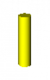
An Internode will be represented as a yellow cylinder. The length and width of the Internode will be specified inside the module, using the constants we defined above.
module Internode extends Organ
{
    double width;

    {
        length = INTERNODE_LENGTH;
        width = INTERNODE_WIDTH;
    }
}
==>
    Cylinder(length, width/2).(setShader(YELLOW))
;
For a leaf, we will start with a very simple representation. It will be made of a petiole (a green cylinder) and a rectangular blade. A turtle command RL will be used to specify the angle of the leaf to the plant stem.
module Leaf extends Organ
{
    double width;
    double angle;
    double petioleLength;
    double petioleWidth;

    {
        length = LEAF_LENGTH;
        width = 0.5*LEAF_LENGTH;
        angle = LEAF_ANGLE;
        petioleLength = 0.2*LEAF_LENGTH;
        petioleWidth = PETIOLE_WIDTH;
    }
}
==>
    RL(angle)
    // petiole
    Cylinder(petioleLength, petioleWidth/2).(setShader(GREEN))
    // leaf blade
    Parallelogram(length-petioleLength, width)
;
Truss will be made of multiple fruits (NB_FRUITS), each represented by a red sphere, connected to the main segments of the truss (yellow cylinders) by small segments (blue cylinders). Different colours are used to help with understanding how the segments carrying the fruits are specified in the code. Turtle commands RL, RH, and RU will be used to add some curvature to the segments of the truss and to place the fruits left and right of the main segments of the truss. (In the truss figure, the individual segments are slightly longer than specified in the code example, for illustration purpose.)
module Truss extends Organ
{
    {length = TRUSS_LENGTH;}
}
==>
    RL(TRUSS_ANGLE) RH(90)
    for (int i:1:NB_FRUITS) (
        Cylinder(length/NB_FRUITS,0.001).(setShader(YELLOW))
        [
            if(i%2==0) (
                RH(90)
            ) else (
                RH(-90)
            )
            RU(60)
            Cylinder(0.02,0.001).(setShader(BLUE))
            // fruit
            Sphere(FRUIT_RADIUS).(setShader(RED))
        ]
        RU(-20)
    )
;
The initial condition
The initial structure, the axiom, is an apex.
protected void init()
[
    Axiom ==> Apex;
]
Rewriting rules
Now we can specify rewriting rules for apex.
First, we specify rewriting rules for vegetative development of the primary shoot in tomato.
public void run()
[
    a:Apex ==>
        Internode
        [Leaf]
        RH(PHYLLOTAXIS_ANGLE)
        a
    ;
]
The turtle command RH is used to create the phyllotactic pattern of leaves (resulting in their placement around the stem).
Now that we have specified the Axiom inside the init() method and a rewriting rule for the Apex inside the run() method, we can run the model by clicking on the run button in the RGG Toolbar, placed above the 3D View.
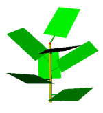
By applying the above rule to an apex 7 times, we create a small plant made of 7 internodes and 7 leaves.
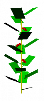
In tomato, after a certain number of phytomers (internodes with leaves), specified by a parameter NB_VEG_PHYTOMERS, primary shoot turns into a sympodial shoot, that bears trusses with fruits. For this sympodial shoot, a repetitive pattern with 3 leaves and 1 truss with fruits is typical in many (high-wire) tomato cultivars.
We first specify a new parameter for the number of phytomers in primary shoot:
const int NB_VEG_PHYTOMERS = 8;
Afterwards, we can add a condition inside our rule, as a switch between primary shoot and sympodial shoot.
public void run()
[
    a:Apex ==>
        Internode
        // in primary shoot, every internode has a leaf
        if (a[rank] <= NB_VEG_PHYTOMERS) (
            [Leaf]
        // in sympodial shoot, only the first in every four
        // internodes has a truss, otherwise it has a leaf
        ) else (
            if ((a[rank] - NB_VEG_PHYTOMERS) % 4 == 1) (
                [Truss]
            ) else (
                [Leaf]
            )
        )
        RH(PHYLLOTAXIS_ANGLE)
        a
        {a[rank]++;}
    ;
]
Note, that in this simple model, we assumed that tomato plants don't form side shoots (in the greenhouse production of high-wire tomatoes, the side shoots are normally removed).
Improving leaf structure
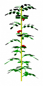
Having captured the basic architecture of tomato plants, we can now improve the leaf structure. Tomato has a composed leaf, with a number of leaflet pairs and a terminal leaflet. We also add leaf curvature, by slightly bending down each segment of the leaf.
const int NB_LEAFLET_PAIRS = 3;
module Leaf extends Organ
{
    ...
}
==>
    RL(angle)
    // petiole
    Cylinder(petioleLength, petioleWidth/2).(setShader(GREEN))

    { double segmentLength = (length-petioleLength)/(NB_LEAFLET_PAIRS+1); }

    // leaflet pairs
    for (int i:1:NB_LEAFLET_PAIRS) (
        [RU(-80) RL(-30) Cylinder(0.04, 0.003) RL(40) Parallelogram(0.1, 0.05)]
        [RU( 80) RL(-30) Cylinder(0.04, 0.003) RL(40) Parallelogram(0.1, 0.05)]
        RL(20)
        Cylinder(segmentLength, 0.003)
    )
    // terminal leaflet
    Parallelogram(segmentLength, 0.05)
;
Improving leaflet shape
So far, we used a simple parallelogram to approximate the shape of a leaflet. We can further refine the leaflet shape, for example by using a MeshNode instead.
For an example on how to generate a leaflet mesh, see the tutorial Leaf triangulation .
We use the code from the leaf triangulation tutorial to create a leaflet mesh MeshNode.(setPolygons(polygonMesh)), where the polygons (polygonMesh) are created from a list of predefined vertices (vertexDataLeaflet).
To use the leaflet mesh in our tomato model, we create a new module for leaflet:
module Leaflet(double length)
==>
    RL(90) Scale(length, length, 0.01) MeshNode.(setPolygons(polygonMesh), setShader(GREEN))
;
Then we replace Parallelogram-s in the Leaf module by the newly defined Leaflet-s:
module Leaf extends Organ
{
    ...
}
==>
    ...

    // leaflet pairs
    for (int i:1:NB_LEAFLET_PAIRS) (
        [RU(-80) RL(-30) Cylinder(0.04, 0.003) RL(40) Leaflet(0.1)]
        [RU( 80) RL(-30) Cylinder(0.04, 0.003) RL(40) Leaflet(0.1)]
        RL(20)
        Cylinder(segmentLength, 0.003)
    )
    // terminal leaflet
    Leaflet(segmentLength)
;

Leaf triangulation
Triangulation is the process where a (ordered) set of triangles is generated out of a (unordered) set of points. The result is a set of triangles, now called faces, that can be directly drawn.
Let's see the following set of 2D point:
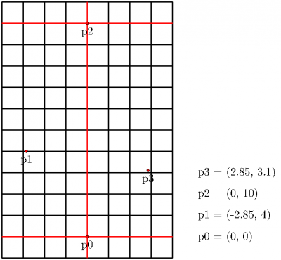
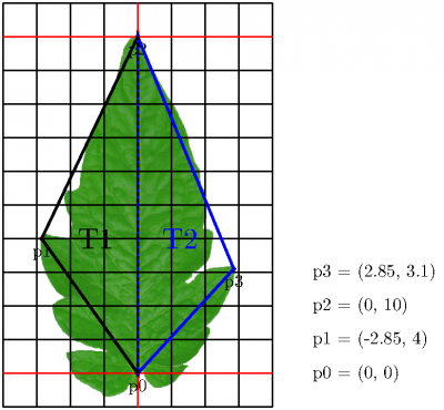
s={(0, 0), (-2.85, 4), (0, 10), (2.85, 3.1)}
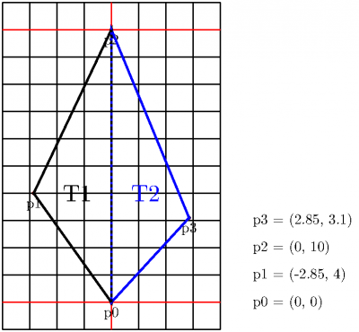
When connecting the points (P_0, P_1, P_2) and (P_1, P_3, P_2) we obtain two triangles. And by doing so, we already did our first (2D) triangulation. In computer graphics such a set of triangles - from now on called faces - is called mesh.
Note: Triangulation is not unique. Meaning there can be different triangulations for the same set of points.
To draw a mesh in GroIMP, all we need to do is to define the point and the faces. The used geometrical object we need to visualize the so-called MeshNode.
The code to generate a simple two faces mesh could look like this:
import de.grogra.xl.util.IntList;
import de.grogra.xl.util.FloatList;

const float[] p0 = {0,0,0};
const float[] p1 = {-2.85,4,0};
const float[] p2 = {0,10,0};
const float[] p3 = {2.85,3.1,0};

const FloatList vertexDataLeaflet = new FloatList(new float[] {
//left
p0[0], p0[1], p0[2], p1[0], p1[1], p1[2], p2[0], p2[1], p2[2],//T1
//right
p0[0], p0[1], p0[2], p2[0], p2[1], p2[2], p3[0], p3[1], p3[2]//T2
});

const PolygonMesh polygonMesh = new PolygonMesh();
static {
    int[] tmp = new int[vertexDataLeaflet.size()/3];
    for(int i = 0; i<tmp.length; i++) tmp[i]=i;
    // set a list of the indices of the used list of vertices
    // normally = {0,1,2,3,...,n}, where n is the number of used vertices minus one
    polygonMesh.setIndexData(new IntList(tmp));
    // set the list of vertices
    polygonMesh.setVertexData(vertexDataLeaflet);
}

protected void init() [
    Axiom ==> Scale(0.007)  MeshNode.(setPolygons(polygonMesh), setShader(GREEN));
]
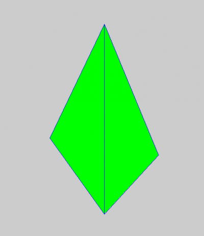
The output of the above code could then look like this. Note: The blue lines to highlight the edges are just added to increase understanding - they will be not shown when running the above code.:
For convex shapes, the Library function leaf3d can be used to generate a triangulation like the above one. It assumes that the first point is the origin of all faces and builds a series of triangles from this point on. In XL this could look like this:
const float[] pointlist = new float[] {0,0,0,-2.85,4,0,0,10,0,2.85,3.1,0};

protected void init() [
	Axiom ==> leaf3d(pointlist);
]
Coming back to the PolygonMesh version, the Library function getMesh takes a FloatList of triangulated points and does the whole conversion to PolygonMesh and MeshNode for us.
static MeshNode LeafletMesh;
static {
    LeafletMesh = getMesh(vertexDataLeaflet);
}

protected void init() [
    Axiom ==> Scale(0.007) LeafletMesh.(setShader(GREEN));
]
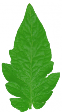
Now, let's take a tomato leaflet for example,
and when placed behind our points, the above triangulation could be already a very rough simplification of this particular leaflet.
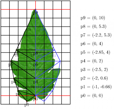
Well, a very rough indeed. So, let's add some more points and also add the the third dimension to give the leaflet some 3D shape.
For the seek of laziness/simplification, the right side of triangles is assumed to be mirror symmetric to the left hand side.
To do so within GroIMP, we just need to add the new points and apply some values for the Z-dimension. A simple curve like this may do:
The complete code to generate the leaflet mesh looks like this:
import de.grogra.xl.util.IntList;
import de.grogra.xl.util.FloatList;

const float[] p0 = {0,0,0};
const float[] p1 = {-0.1,-0.066,0.3};
const float[] p2 = {-0.2,0.06,0};
const float[] p3 = {-0.25,0.2,0};
const float[] p4 = {0,0.2,-0.4};
const float[] p5 = {-0.285,0.4,0};
const float[] p6 = {0,0.4,-0.5};
const float[] p7 = {-0.22,0.53,0};
const float[] p8 = {0,0.53,-0.3};
const float[] p9 = {0,1,1.0};

const FloatList vertexDataLeaflet = new FloatList(new float[] {
//left
p0[0], p0[1], p0[2], p1[0], p1[1], p1[2], p2[0], p2[1], p2[2],//T1
p0[0], p0[1], p0[2], p2[0], p2[1], p2[2], p3[0], p3[1], p3[2],//T2
p0[0], p0[1], p0[2], p3[0], p3[1], p3[2], p4[0], p4[1], p4[2],//T3
p3[0], p3[1], p3[2], p4[0], p4[1], p4[2], p5[0], p5[1], p5[2],//T4
p4[0], p4[1], p4[2], p5[0], p5[1], p5[2], p6[0], p6[1], p6[2],//T5
p5[0], p5[1], p5[2], p6[0], p6[1], p6[2], p7[0], p7[1], p7[2],//T6
p6[0], p6[1], p6[2], p7[0], p7[1], p7[2], p8[0], p8[1], p8[2],//T7
p7[0], p7[1], p7[2], p8[0], p8[1], p8[2], p9[0], p9[1], p9[2],//T8
//right
-p0[0], p0[1], p0[2], -p1[0], p1[1], p1[2], -p2[0], p2[1], p2[2],//T9
-p0[0], p0[1], p0[2], -p2[0], p2[1], p2[2], -p3[0], p3[1], p3[2],//T10
-p0[0], p0[1], p0[2], -p3[0], p3[1], p3[2], -p4[0], p4[1], p4[2],//T11
-p3[0], p3[1], p3[2], -p4[0], p4[1], p4[2], -p5[0], p5[1], p5[2],//T12
-p4[0], p4[1], p4[2], -p5[0], p5[1], p5[2], -p6[0], p6[1], p6[2],//T13
-p5[0], p5[1], p5[2], -p6[0], p6[1], p6[2], -p7[0], p7[1], p7[2],//T14
-p6[0], p6[1], p6[2], -p7[0], p7[1], p7[2], -p8[0], p8[1], p8[2],//T15
-p7[0], p7[1], p7[2], -p8[0], p8[1], p8[2], -p9[0], p9[1], p9[2]//T16
});

static MeshNode LeafletMesh;
static {
    LeafletMesh = getMesh(vertexDataLeaflet);
}

protected void init() [
    Axiom ==> Scale(0.07, 0.07, 0.01) LeafletMesh.(setShader(GREEN));
]
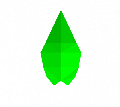
The output of the above code could then look like this:
The last step would now be to pack the leaflet mesh into a module and integrate it further into a leaf module (not shown here). For the first aspect, we can define a module like this:
module Leaflet(float length) ==>
    Scale(length, length, 0.01) MeshNode.(setPolygons(polygonMesh), setShader(GREEN));
After integration in to a leaf module the final 3D result could look like this
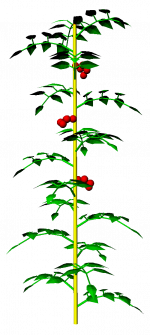
as it was used within Zhang et al. 2021 (High resolution 3D simulation of light climate and thermal performance of a solar greenhouse model under tomato canopy structure; Renewable Energy, 160, 730-745, doi: https://doi.org/10.1016/j.renene.2020.06.144).
GroIMP provides a few predefined 3D leaves that can be accessed using the Library function leaf3d(id). There are shapes for: “artificial”, “maple”, “undefined”, “poplar”, “cotton”, “birch”, “undefined”, “oak”. The identifier starts from zero for the first “artificial” shape and goes up to seven for the oak leaf.
The code below will generate them one by one next to each other.
protected void init() [
  Axiom ==>
    for(int i=0; i<DEFAULT_LEAF3D.length; i++) (
      [ Null(i*0.3,0,0) leaf3d(i) ]
    )
]
The predefined 3D leaf shapes will look as shown below:
General Introduction
Rendering vs Light Modelling
Rendering is the process of generating a (final) image (or a series of images) from a 3D scene. This includes computing how surfaces appear based on materials, lighting, camera position, and other visual effects.
Light Modelling refers to the mathematical and physical simulation of how light behaves in a 3D environment, particularly how it interacts with objects (reflection, refraction, absorption, scattering).
| Feature | Rendering | Light Modelling |
|---|---|---|
| Goal | Create image | Simulate realistic light behaviour |
| Focus | Visual output | Physical correctness and realism |
| Includes | Shading, camera, rasterization | Reflection, refraction, light transport |
Light Modelling
Light modelling generally involves three aspects:
- Global illumination model
- Light sources
- Local illumination model
Whereas the Global illumination model handles the actual light computation, the Light sources are the light-emitting elements, and the Local illumination model defines the optical properties of the scene objects.
In each aspect, computer graphics offers plenty of alternatives.
Several of them are implemented in GroIMP as ready-to-use tools.
GroIMP integrates two main light model implementations, namely:
- Twilight, a CPU-based implementation
- GPUFlux, a GPU-based implementation
Both implementing different global illumination model for rendering and for light computation.
More on the different ways to implement a global illumination model can be found here: Ray tracer algorithm
The general settings of the can be changed within the GroIPM properties as described in the Ray tracer options section.
In the following, only light computation or light modelling will be discussed.
Regarding light sources, GroIMP provides a complete set of possible implementations. They all implement the Light and LightBase interfaces, which makes them easy to handle and exchange.
For the Local illumination model, which defines the optical properties of the scene objects such as values for absorption, transmission, and reflection, so-called shaders are used.
GroIMP provides a set of standard shader implementations, e.g., for Lambert and Phong shading. Whereas the Lambertian model supports only diffuse reflection, the Phong reflection model (Phong, 1973) combines ambient, diffuse, and specular light reflections.
References
Phong BT, Illumination of Computer-Generated Images, Department of Computer Science, University of Utah, UTEC-CSc-73-129, July 1973.
First steps on light modelling
This tutorial we show you the basics on how to do light modelling in GroIMP.
For some more theoretical background pleas refer to the Introduction - A little bit of Theory page. For an advanced tutorial on spectral light modelling check out the Spectral light modelling tutorial.
GroIMP integrates two two main light model implementations, namely:
- Twilight, a CPU-based implementation
- GPUFlux, a GPU-based implementation
While they are both integrating various renderer and light model implementations, they differ in a few details we are not gonna be discuss here. Please refer to the Differences between the CPU and GPU light model page for details. The two main difference however are first that the GPU implementation is several times faster than the CPU implementation and second, that the GPU version is, beside the three channel RGB implementation, able to simulate the full visible light spectrum (spectral light modelling).
In the following, we focus on the three channel RGB versions of both the CPU and GPU implementations.
To set up a light model basically three steps are needed.
- Definition/Initialization of the light model
- Running the light model
- Checking the scene objects for their light absorption
In GroIMP/XL, this can be done as following:
For the Twilight (CPU-based) implementation:
import de.grogra.ray.physics.Spectrum;

//constants for the light model: number of rays and maximal recursion depth
const int RAYS = 1000000;
const int DEPTH = 10;

//initialize the scene
protected void init() {

  //create the actual 3D scene
  [
    Axiom ==> Box(0.1,1,1).(setShader(BLACK)) M(2) RL(180)
    LightNode.(setLight(new SpotLight().(setPower(100),setInnerAngle(0.02),setOuterAngle(0.055))));
  ]

  //make sure the changes on the graph are applied...
  {derive();}
  //so that we directly can continue and work on the graph


  // initialize the light model
  LightModel CPU_LM = new LightModel(RAYS, DEPTH);

  CPU_LM.compute(); // run the light model

  //check the scene objects for their light absorption
  Spectrum ms;
  [
    x:Box::> { ms = CPU_LM.getAbsorbedPower(x); }
  ]
  print("absorbed = "+ms);println(" = "+ms.integrate(), 0xff0000);
}
Direct after saving the code, the light model will be executed and the following will be printed in the XL Console Window:
While in the above example the object is black, what means that all incoming radiation is absorbed (and nothing reflected), the line below will shange the object colour to some orange
Axiom ==> Box(0.1,1,1).(setShader(new RGBAShader(1,0.5,0))) M(2) RL(180)
what means that all of red and 50% of green are reflected while all blue radiation is absorbed as the resulting output confirms.
For the GPUFlux (GPU-based) implementation:
import de.grogra.gpuflux.tracer.FluxLightModelTracer.MeasureMode;
import de.grogra.gpuflux.scene.experiment.Measurement;

//constants for the light model: number of rays and maximal recursion depth
const int RAYS = 1000000;
const int DEPTH = 10;

//initialize the scene
protected void init() {

  //create the actual 3D scene
  [
    Axiom ==> Box(0.1,1,1).(setShader(BLACK)) M(2) RL(180)
        LightNode.(setLight(new SpotLight().(setPower(100),setInnerAngle(0.02),setOuterAngle(0.055))));
  ]

  //make sure the changes on the graph are applied...
  {derive();}
  //so that we directly can continue and work on the graph


  // initialize the light model
  FluxLightModel GPU_LM = new FluxLightModel(RAYS, DEPTH);
  GPU_LM.setMeasureMode(MeasureMode.RGB); // user the Flux model in three channel 'RGB mode'
  //GPU_LM.setMeasureMode(MeasureMode.FULL_SPECTRUM);
  //GPU_LM.setSpectralDomain(300,800);// spectral range monitored
  //GPU_LM.setSpectralBuckets(31);// range divided into 30 buckets

  GPU_LM.compute(); // run the light model

  //check the scene objects for their light absorption
  Measurement ms;
  [
    x:Box::> { ms = GPU_LM.getAbsorbedPowerMeasurement(x); }
  ]
  print("absorbed = "+ms);println(" = "+ms.integrate(), 0xff0000);
}
For details on spectral light modelling, please refer to Spectral light modelling

